Countdown
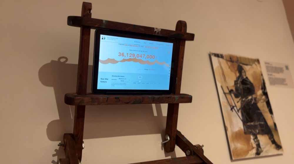
website
Online realtime GHG (Green House Gases) emission counter produced by World Data Lab.
OpenAI. (2026). ChatGPT (GPT-5.6) [Large language model]. See prompts at the end
World Emissions Clock
Institutional genealogy, data reliability and the history of greenhouse-gas measurement
Scope: The World Emissions Clock website and its institutional background, launch history, current methodology and appropriate uses; a concise history of atmospheric greenhouse-gas measurement and emissions accounting; and a source-critical audit and visualisation of the user-supplied Atmospheric CO₂ Concentration (1850–2024) dataset. The report does not independently reproduce all 12,000-plus country-sector scenario trajectories.
Abstract
Launched at COP27 on 18 November 2022, the World Emissions Clock is a World Data Lab and Vienna University of Economics and Business project developed with German development institutions, IIASA, Oxford and philanthropic support. It now presents historical estimates and three conditional pathways for 182 countries, five main sectors and up to 24 subsectors through 2050. Its historical base and business-as-usual model draw on reputable datasets and a peer-reviewed econometric framework. The display is nevertheless not a live atmospheric measurement: after the latest historical anchor, the ticking values are modelled and continuously interpolated. Country-sector estimates also inherit uncertainty from emission factors, scenario assumptions, downscaling, land-use accounting and the conversion of non-CO₂ gases into 100-year CO₂ equivalents. The attached 1850–2024 CO₂ concentration file is not an authentic annual observational series: it consists of two exact linear trends separated by a 13.95 ppm discontinuity and diverges materially from NOAA records. For The Sunshine Find, the Clock is best understood as a panoptic climate dashboard: it turns dispersed industrial activity into an apparently immediate global spectacle while obscuring the interpretive decisions required to make emissions countable.
Project links and cross-references: Project website · Exhibition objects · Archive of global-warming narratives. Read especially beside Countdown (object 21), The Random Archive, Discovery of Global Warming, Future, Drill baby, drill!, SUVization and The cloud is not in the sky!.
Contents
1. Object and institutional background
2. What the Clock counts: data architecture and scenarios
3. Reliability assessment
4. From gases to global networks: a history of measurement
5. From concentration to emissions: inventories, models and near-real-time estimates
6. Audit of the attached Atmospheric CO₂ 1850–2024 dataset
7. Primary and institutional evidence
8. Numbered academic reference list
Appendix: User prompts related to this report
1. Object and institutional background
The World Emissions Clock (WEC) belongs to a family of public-facing “clocks” that translate large statistical systems into a continuously changing number. It is not a separate observatory or intergovernmental inventory. It is an online modelling and communication project led by World Data Lab (WDL) in cooperation with the Vienna University of Economics and Business (WU). WDL traces its institutional origin to a 2014 data-democratisation initiative founded by economists Homi Kharas and Wolfgang Fengler; the organisation subsequently combined public-interest “clock” projects with commercial forecasting products.
Field | Documented information |
Public launch | 18 November 2022, during COP27 in Sharm el-Sheikh, Egypt. |
Lead organisations | World Data Lab; Vienna University of Economics and Business (WU). |
Named development partners at launch | German Federal Ministry for Economic Cooperation and Development (BMZ); Deutsche Gesellschaft für Internationale Zusammenarbeit (GIZ); Patrick J. McGovern Foundation; International Institute for Applied Systems Analysis (IIASA); University of Oxford. |
Scientific leadership | The launch announcement names WU professor Jesús Crespo Cuaresma as scientific lead for the statistical model; the peer-reviewed framework was published by Lukas Vashold and Crespo Cuaresma in 2024. |
Launch coverage | 180 countries, five main sectors and up to 24 subsectors to 2050. |
Current stated coverage | 182 countries, up to 24 subsectors, international aviation and shipping, and more than 12,000 sectoral trajectories to 2050. |
Mission | To make historical emissions, policy commitments and 1.5°C-compatible pathways comparable and actionable through the concepts of an “implementation gap” and an “ambition gap”. |
Academic source links: Peer-reviewed BAU modelling framework | Synthetic historical GHG dataset
References: [1], article 139; [2], 5213–5252.
Primary / institutional evidence links: WU launch announcement | World Emissions Clock methodology | World Data Lab institutional history
The expansion from 180 countries at launch to 182 on the current methodology page is documented, but the public pages reviewed do not identify a precise date for that coverage change. The wording “clock” should therefore be read as interface design, not as evidence of a continuously observing instrument.
2. What the Clock counts: data architecture and scenarios
The site displays greenhouse-gas emissions as mass flows in tonnes of CO₂ equivalent (CO₂e). This is conceptually different from atmospheric concentration, which is measured as a mole fraction in parts per million or billion. Emissions describe how much gas enters or leaves the atmosphere over time; concentration describes how much is present in an air sample. The two are connected through the carbon cycle and atmospheric chemistry but are not interchangeable.
Clock layer | Method and source |
Historical emissions before 2022 | The Minx et al. synthetic dataset, built principally from EDGAR and covering anthropogenic CO₂, CH₄, N₂O and fluorinated gases by sector. |
2022–2023 update | The current methodology says sectoral dynamics are extended with EDGAR data. |
Business as usual after 2023 | A country- and sector-level time-series/econometric model using historical emission intensities, GDP, population, demography, urbanisation, SSP2 pathways and IMF short-term forecasts. |
“Do as we promised” | A pathway applying unconditional Nationally Determined Contributions; EU member states inherit the EU-level NDC even where national plans are more stringent. |
“We achieve the goal” | A globally cost-efficient 1.5°C pathway derived from IIASA/NGFS integrated assessment modelling, primarily MESSAGE-GLOBIOM for CO₂ and GAINS for non-CO₂ gases. |
Country downscaling | Regional IAM results are distributed to countries using energy mix, development, demographic and sector-specific variables. |
Land use and forestry | Excluded from the core time-series forecast; derived separately by downscaling MESSAGE-GLOBIOM and reconciling IAM totals with country-reported/PRIMAP information. |
Common unit | 100-year Global Warming Potentials convert non-CO₂ gases into CO₂e. |
Academic source links: Vashold and Crespo Cuaresma, modelling framework | Minx et al., historical dataset | Lamb et al., why GHG totals differ
References: [1], article 139; [2], 5213–5252; [3], 2549–2572.
Primary / institutional evidence links: Current methodology and glossary | EDGAR emissions database | NGFS climate scenarios
The apparent second-by-second movement is therefore an interpolation of annual or scenario-based rates. It does not mean that instruments are directly measuring every emitted tonne as it leaves a source. The interface turns a modelled flow into a present-tense visual event.
3. Reliability assessment
Reliability depends on the question. The Clock is strongest as a comparative and pedagogical interface, weaker as a source for exact country-year numbers, and inappropriate as a stand-alone compliance or forensic record.
Use / dimension | Assessment |
Historical global and broad sector trends | Strong to moderate. EDGAR and the Minx synthesis are reputable, standardised and transparent, but they remain bottom-up estimates rather than complete direct observations. |
Cross-country comparability | Moderate to strong at broad scale. Harmonised assumptions improve comparison; they may also diverge from national inventories using country-specific data and higher-tier methods. |
Business-as-usual projection | Moderate as a benchmark, not a forecast of the “most likely” future. The peer-reviewed paper explicitly conditions results on an SSP2 narrative and treats uncertainty bands as lower bounds. |
NDC and 1.5°C pathways | Conditional scenarios, not predictions. Only unconditional NDCs are represented, and the 1.5°C display selects one cost-efficient pathway from a larger scenario family. |
Country/subsector precision | Moderate to low for high-stakes use. Regional-to-country downscaling, regression shares, imputations and ex-post corrections add uncertainty. |
Land-use, land-use change and forestry | Low to moderate. The site itself warns of large uncertainties and conceptual incompatibilities between inventories and IAMs. |
Non-CO₂ aggregation | Useful but convention-dependent. A 100-year GWP conceals the different lifetimes and near-term effects of methane, nitrous oxide and fluorinated gases. |
“Real-time” status | Low if interpreted literally. The display is modelled and interpolated; it is not a sensor network or a continuously verified global inventory. |
Policy, legal or facility attribution | Unsuitable alone. Exact claims should be checked against UNFCCC inventories, EDGAR, national statistics, facility monitoring, Global Carbon Budget datasets and, where relevant, atmospheric inversions or source-detection systems. |
Academic source links: Uncertainty and system boundaries in GHG estimates | BAU framework and uncertainty limits | Historical dataset and uncertainty assessment
References: [1], article 139; [2], 5213–5252; [3], 2549–2572.
A further transparency issue is visual rather than statistical. The methodology acknowledges considerable uncertainty but deliberately abstracts from it to preserve an accessible interface. The single moving figure consequently appears more determinate than the underlying evidence warrants. This is not falsification; it is a communicative compression whose limits must remain visible.
4. From gases to global networks: a history of measurement
The history of greenhouse-gas measurement combines three distinct developments: identifying gases chemically; determining how they absorb radiation; and measuring their atmospheric abundance with sufficient precision, calibration and spatial coverage. Several famous climate scientists contributed mainly to theory rather than to atmospheric sampling, so their roles should not be conflated.
Period / contributor | Methodological contribution |
1750s — Joseph Black | Identified “fixed air” (carbon dioxide) as a chemically distinct gas through gravimetric and reaction-based experiments. This established that air is a mixture rather than a single substance. |
Late eighteenth–early nineteenth century — Horace-Bénédict and Nicolas-Théodore de Saussure | Developed eudiometric and absorption-based approaches to air analysis and linked atmospheric CO₂ to plant carbon assimilation. Early measurements were local and method-sensitive. |
1824–1827 — Joseph Fourier | Developed a physical account of planetary heat balance and atmospheric insulation. Fourier did not measure greenhouse-gas concentration; his contribution was theoretical. |
1856 — Eunice Newton Foote | Compared solar heating in glass cylinders containing different gases. Her simple thermometer experiment showed enhanced warming in carbonic-acid gas and moist air, but did not measure infrared spectra. |
1859–1861 — John Tyndall | Used a long gas tube, a differential thermopile and infrared radiation to measure the selective absorption and emission of heat by water vapour, CO₂ and other gases. This provided laboratory spectroscopy of greenhouse behaviour. |
Mid-to-late nineteenth century — Max von Pettenkofer method | Standardised wet-chemical CO₂ analysis through alkaline absorption and titration. It enabled many measurements but was vulnerable to siting, contamination, reagent and calibration differences. |
1896 — Svante Arrhenius | Combined radiative calculations, spectral knowledge and early CO₂ estimates to quantify the temperature response to changing atmospheric carbonic acid. This was calculation rather than a monitoring network. |
1938 — Guy Stewart Callendar | Selected and compared historical chemical CO₂ measurements with fossil-fuel production and temperature records, arguing that atmospheric CO₂ was rising. Later reassessment showed why heterogeneous nineteenth-century measurements require strict quality control. |
1950s–1960s — Charles David Keeling | Introduced high-precision manometric calibration, stable reference gases and continuous non-dispersive infrared analysis. Measurements at the South Pole and Mauna Loa revealed both the seasonal cycle and sustained anthropogenic rise. |
1957 onward — global flask and in-situ networks | Discrete air samples, calibrated in-situ analysers and international reference scales expanded monitoring beyond single stations. Intercomparability became as important as instrument sensitivity. |
1960s–2000s — polar ice-core teams | Crushed or melted ice under vacuum to extract ancient air, then measured CO₂, CH₄ and N₂O with gas chromatography, infrared analysis and mass spectrometry. Corrections for gas age, ice age, diffusion and enclosure processes made paleoclimate reconstructions possible. |
Late twentieth century to present — laser and Fourier-transform spectroscopy | Cavity ring-down, tunable-diode-laser and FTIR systems improved precision and allowed continuous multi-gas observations, including isotopic measurements useful for source attribution. |
1990s to present — satellite remote sensing | Thermal- and near-infrared spectrometers progressed from experimental trace-gas retrievals to dedicated greenhouse-gas missions such as GOSAT and OCO-2, producing column-averaged concentration fields with global repeat coverage. Satellites complement rather than replace surface calibration networks. |
Academic source links: Historical development of climate science | Foote and Tyndall priority study | Keeling measurement history | Law Dome ice-core records | Satellite trace-gas spectroscopy
References: [4]; [5], 105–118; [6], 1–36; [7], 237–276; [8], 223–240; [9], 87–105; [10], 7865–7870; [11], 200–203; [12], 538–551; [13], 4115–4128; [14], article L14810; [15], 379–382; [16], 1495–1508; [17], 700–709.
5. From concentration to emissions: inventories, models and near-real-time estimates
Atmospheric instruments measure concentrations and isotopic composition. They do not by themselves assign every molecule to a country, sector or company. Emissions accounting therefore developed as a parallel system that combines statistics, engineering measurements and atmospheric modelling.
Method | How it works and what it can establish |
Bottom-up inventories | Activity data — fuel burned, clinker produced, livestock numbers, fertiliser use, refrigerant stocks or land-use change — are multiplied by emission factors or process models. IPCC tiers range from generic defaults to country- and facility-specific methods. |
Direct source and stack monitoring | Flow, gas concentration and process parameters are measured at installations, often continuously for regulated pollutants and major combustion sources. Coverage varies by jurisdiction and source type. |
National reporting | Inventories aggregate territorial sources under UNFCCC categories. Reporting timetables, capacity and methodological tiers differ, so the latest complete year may lag the present. |
Independent harmonised databases | EDGAR and related syntheses apply common methods across countries to improve comparability, accepting that results may differ from national submissions. |
Top-down atmospheric inversions | Surface, aircraft and satellite concentration observations are combined with atmospheric transport models to infer the spatial distribution of net sources and sinks. These estimates are particularly important for methane and land carbon, but depend on transport, prior estimates and network density. |
Near-real-time proxies | Electricity generation, traffic, industrial production and mobility indicators can estimate daily or monthly fossil CO₂ changes before official inventories are complete. Carbon Monitor demonstrates the method but also illustrates that “near-real-time” remains estimation, not a complete direct census. |
Scenario projection | Econometric and integrated assessment models extend historical relationships under explicit socioeconomic, technological and policy assumptions. The World Emissions Clock belongs primarily to this layer after its historical anchor. |
Academic source links: Minx et al., bottom-up synthesis | Lamb et al., inventory conventions | Carbon Monitor near-real-time dataset | Global Carbon Budget 2024
References: [2], 5213–5252; [3], 2549–2572; [18], article 392; [19], 965–1039.
Primary / institutional evidence links: 2006 IPCC inventory guidelines | 2019 IPCC refinement | UNFCCC reporting and review | WMO Global Atmosphere Watch
6. Audit of the attached Atmospheric CO₂ 1850–2024 dataset
The user-supplied document labels its values “Atmospheric CO₂ Concentration” and states that pre-1958 values are reconstructed from ice cores while post-1958 values are direct Mauna Loa measurements. Its cited sources are credible, but the numbers in the table do not reproduce those sources. The dataset appears to be a schematic interpolation assembled from two straight lines.
Test | Result |
Data type | Atmospheric concentration in ppm. It is not a dataset of GHG emissions and therefore cannot be plotted as evidence for the World Emissions Clock’s tonne-per-second counter. |
1850–1957 pattern | Every annual increment is exactly +0.15 ppm. Real ice-core reconstructions are not a perfect arithmetic progression and have temporal-resolution and smoothing limits. |
1957–1958 transition | The table jumps from 301.05 to 315.0 ppm: +13.95 ppm in one year. This is a splice artefact, not a plausible global atmospheric change. |
1958–2024 pattern | Every annual increment is exactly +1.60 ppm. The actual Mauna Loa growth rate varies from year to year and accelerates over the record. |
Start of annual Mauna Loa means | NOAA’s complete annual-mean series begins in 1959; measurements started in March 1958, so 1958 is not a complete annual mean in the standard NOAA table. |
Error against NOAA Mauna Loa, 1959–2024 | Mean absolute error 8.59 ppm; root-mean-square error 9.49 ppm. |
Largest absolute difference | 1993: attached 371.00 ppm versus NOAA Mauna Loa 357.21 ppm, a +13.79 ppm difference. |
2024 comparison | Attached 420.60 ppm; NOAA Mauna Loa 424.61 ppm; NOAA globally averaged marine-surface value 422.79 ppm. |
Editorial status | Do not describe the attached table as a “full yearly dataset” based on NOAA or ice-core observations. Retain it only as a visibly labelled schematic, or replace it with the original NOAA/global and ice-core series. |
Academic source links: Keeling’s early atmospheric record | Mauna Loa measurement programme | Law Dome ice-core reconstruction | Global Carbon Budget 2024
References: [11], 200–203; [12], 538–551; [13], 4115–4128; [19], 965–1039.
Primary / institutional evidence links: NOAA Mauna Loa annual means | NOAA globally averaged annual means | NOAA Trends in Atmospheric Carbon Dioxide
Figure 1. Atmospheric CO₂ concentration, 1850–2024. The attached series is plotted against NOAA Mauna Loa and globally averaged annual means. Its two straight segments and 1958 discontinuity demonstrate that it is a schematic construction rather than an observational yearly record. Source audit and figure: this report; NOAA data downloaded 27 July 2026.
The graph is intentionally comparative. A graph of the attached values alone would make the piecewise-linear series appear authoritative while concealing its incompatibility with the source named in the document. The comparison turns data criticism into part of the visual evidence.
7. Primary and institutional evidence
1. World Emissions Clock. Public interactive interface.
2. World Emissions Clock methodology. Current coverage, scenarios, inputs, downscaling, harmonisation, uncertainty and glossary.
3. WU launch announcement, 18 November 2022. Launch date, partners, initial scope and mission.
4. World Data Lab institutional history. Organisation’s account of its 2014 origin and development.
5. EDGAR. European Commission Joint Research Centre harmonised global emissions database.
6. NOAA Trends in Atmospheric Carbon Dioxide. Direct atmospheric CO₂ monitoring and downloadable annual means.
7. WMO Global Atmosphere Watch. International observation, calibration and quality-assurance framework.
8. IPCC National Greenhouse Gas Inventory Programme. Inventory guidelines and methodological refinements.
9. UNFCCC greenhouse-gas inventories. National reporting framework and submissions.
10. NGFS climate scenarios portal. Scenario framework used in the WEC’s policy pathways.
8. Numbered academic reference list
Chicago bibliography style. The numbered list contains only scholarly books and peer-reviewed articles. Primary and institutional pages are separated above.
1. Vashold, Lukas, and Jesús Crespo Cuaresma. “A Unified Modelling Framework for Projecting Sectoral Greenhouse Gas Emissions.” Communications Earth & Environment 5 (2024): article 139. https://doi.org/10.1038/s43247-024-01288-9.
2. Minx, Jan C., William F. Lamb, Robbie M. Andrew, Josep G. Canadell, Monica Crippa, Niklas Döbbeling, Piers M. Forster, et al. “A Comprehensive and Synthetic Dataset for Global, Regional, and National Greenhouse Gas Emissions by Sector 1970–2018 with an Extension to 2019.” Earth System Science Data 13 (2021): 5213–5252. https://doi.org/10.5194/essd-13-5213-2021.
3. Lamb, William F., Robbie M. Andrew, Matthew Jones, Zebedee Nicholls, Glen P. Peters, Chris Smith, Marielle Saunois, et al. “Differences in Anthropogenic Greenhouse Gas Emissions Estimates Explained.” Earth System Science Data 18 (2026): 2549–2572. https://doi.org/10.5194/essd-18-2549-2026.
4. Fleming, James Rodger. Historical Perspectives on Climate Change. New York: Oxford University Press, 1998.
5. Jackson, Roland. “Eunice Foote, John Tyndall and a Question of Priority.” Notes and Records: The Royal Society Journal of the History of Science 74, no. 1 (2020): 105–118. https://doi.org/10.1098/rsnr.2018.0066.
6. Tyndall, John. “The Bakerian Lecture: On the Absorption and Radiation of Heat by Gases and Vapours, and on the Physical Connexion of Radiation, Absorption, and Conduction.” Philosophical Transactions of the Royal Society of London 151 (1861): 1–36. https://doi.org/10.1098/rstl.1861.0001.
7. Arrhenius, Svante. “On the Influence of Carbonic Acid in the Air upon the Temperature of the Ground.” The London, Edinburgh, and Dublin Philosophical Magazine and Journal of Science, 5th ser., 41, no. 251 (1896): 237–276. https://doi.org/10.1080/14786449608620846.
8. Callendar, G. S. “The Artificial Production of Carbon Dioxide and Its Influence on Temperature.” Quarterly Journal of the Royal Meteorological Society 64, no. 275 (1938): 223–240. https://doi.org/10.1002/qj.49706427503.
9. From, E., and C. D. Keeling. “Reassessment of Late 19th Century Atmospheric Carbon Dioxide Variations.” Tellus B 38, no. 2 (1986): 87–105. https://doi.org/10.3402/tellusb.v38i2.15083.
10. Harris, Daniel C. “Charles David Keeling and the Story of Atmospheric CO₂ Measurements.” Analytical Chemistry 82, no. 19 (2010): 7865–7870. https://doi.org/10.1021/ac1001492.
11. Keeling, C. D. “The Concentration and Isotopic Abundances of Carbon Dioxide in the Atmosphere.” Tellus 12, no. 2 (1960): 200–203. https://doi.org/10.3402/tellusa.v12i2.9366.
12. Keeling, C. D., R. B. Bacastow, A. E. Bainbridge, C. A. Ekdahl Jr., P. R. Guenther, L. S. Waterman, and J. F. S. Chin. “Atmospheric Carbon Dioxide Variations at Mauna Loa Observatory, Hawaii.” Tellus 28, no. 6 (1976): 538–551. https://doi.org/10.1111/j.2153-3490.1976.tb00701.x.
13. Etheridge, D. M., L. P. Steele, R. L. Langenfelds, R. J. Francey, J.-M. Barnola, and V. I. Morgan. “Natural and Anthropogenic Changes in Atmospheric CO₂ over the Last 1000 Years from Air in Antarctic Ice and Firn.” Journal of Geophysical Research: Atmospheres 101, no. D2 (1996): 4115–4128. https://doi.org/10.1029/95JD03410.
14. MacFarling Meure, C., D. Etheridge, C. Trudinger, P. Steele, R. Langenfelds, T. van Ommen, A. Smith, and J. Elkins. “Law Dome CO₂, CH₄ and N₂O Ice Core Records Extended to 2000 Years BP.” Geophysical Research Letters 33, no. 14 (2006): L14810. https://doi.org/10.1029/2006GL026152.
15. Lüthi, Dieter, Martine Le Floch, Bernhard Bereiter, et al. “High-Resolution Carbon Dioxide Concentration Record 650,000–800,000 Years before Present.” Nature 453 (2008): 379–382. https://doi.org/10.1038/nature06949.
16. Clerbaux, Cathy, Juliette Hadji-Lazaro, Solène Turquety, Gérard Mégie, and Pierre-François Coheur. “Trace Gas Measurements from Infrared Satellite for Chemistry and Climate Applications.” Atmospheric Chemistry and Physics 3 (2003): 1495–1508. https://doi.org/10.5194/acp-3-1495-2003.
17. Crisp, David, R. M. Atlas, F.-M. Bréon, et al. “The Orbiting Carbon Observatory (OCO) Mission.” Advances in Space Research 34, no. 4 (2004): 700–709. https://doi.org/10.1016/j.asr.2003.08.062.
18. Liu, Zhu, Philippe Ciais, Zhu Deng, et al. “Carbon Monitor, a Near-Real-Time Daily Dataset of Global CO₂ Emission from Fossil Fuel and Cement Production.” Scientific Data 7 (2020): article 392. https://doi.org/10.1038/s41597-020-00708-7.
19. Friedlingstein, Pierre, Michael O’Sullivan, Matthew W. Jones, Robbie M. Andrew, Judith Hauck, Peter Landschützer, Corinne Le Quéré, et al. “Global Carbon Budget 2024.” Earth System Science Data 17 (2025): 965–1039. https://doi.org/10.5194/essd-17-965-2025.
Appendix: User prompts related to this report
Prompts are reproduced chronologically as a research-process record. Spelling and punctuation are preserved.
1. Analyse this website: https://worldemissions.io/
1. develop on its background (insitutions, launching dates, mission), research on the reliabilty of its data
2. Summarise the history of measurements methods of GHG throughout the times with notable scientist that contributed to it.
3. create a graph out of the report data attached.
2. General remarks:
1. I have been asking you to create individual reports on different topics.
2. Nonetheless these materials should converge into a unity which is the archive itself and the supporting physical installation. This convergence should be based on a synthesys of all of my other topics, questions and criteria raised in all of the other chat sessions, which are all part of the same project the main scope of which is an art installation and a supporting archive that grows by time. The archive is meant for both professional and nonprofessional use, it should be informative within its artistic and pedagogical scope as well.
3. the main line of thoughts of the project departs from panoptic tourism and concludes to ecoterrorism in a narrative line. Therefore all the reports should follow this general direction in their approach and references.
4. The reports we are working on now will all serve as a background research material published on the project website for the set of objects that will be on display, Each object will have its own page (see: https://glacial-archaeology.net/category/exhibition/). See: Szabolcs KissPál – The sunshine find_for translation. I am also adding the brief description of the project’s general concept, see: Szabolcs KissPál – The sunshine find. The website will have a separate but interconnected section for both the exhibition and the supporting archive. https://glacial-archaeology.net/an-archive-of-narratives-on-global-warming-copy/ Inspect the site while note that it doesn’t have its final structure yet!
5. the scope with the reports is to produce a set of background research material for each object in part that should refer to each other, and should be unified in their narrative and typographic structure, tone, and scope. Pay attention to snychronise the focus points of different partial research tasks when possible with cross references!
6. I am attaching two of your previous reports (noahs_ark_expeditions_1959_1990_academic_sources_new_tab_links.docx, Container_Mount_Scorluzzo_WWI_Shelter_Research_Report). Please develop and and apply to these reports a uniform structure both content wise and in formal aspects while mostly keeping their original content.
7. Main further formal criteria:
– you should always start with an abstract summarizing your finds in a text no longer than 200 words.
– you should always enlist at the very end of the document all my prompts related to that topic
– the external links should always open in a different tab
– you should be using only valid, peer reviewed academic sources listed and numbered at the end of the documents
– you should apply a somewhat unified narrative structured and a unified formatting (including typeface styles, subtitles structure, etc.
8. – note and memorise the above in your cross-chat memory for rurther tasks